Minotaur Plotter

Apr 2026

A C++17 desktop application for converting images into vector paths and driving pen plotters in real time. Compatible with the Axidraw A3 (now Bantam Tools)

Source : https://github.com/nshelton/Minotaur

(theoretically cross platform, but haven’t build on windows for a bit of time). MacOS is supported.

Overview

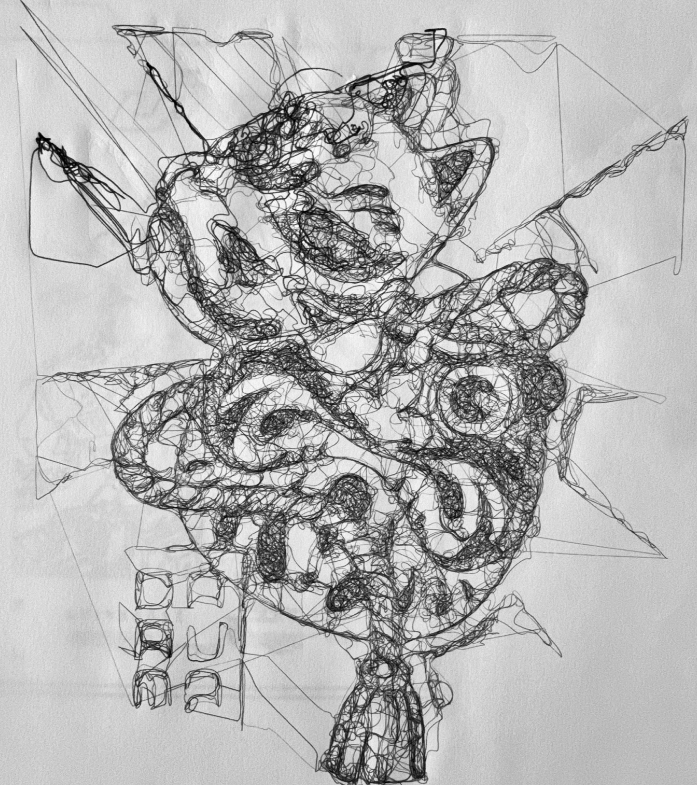
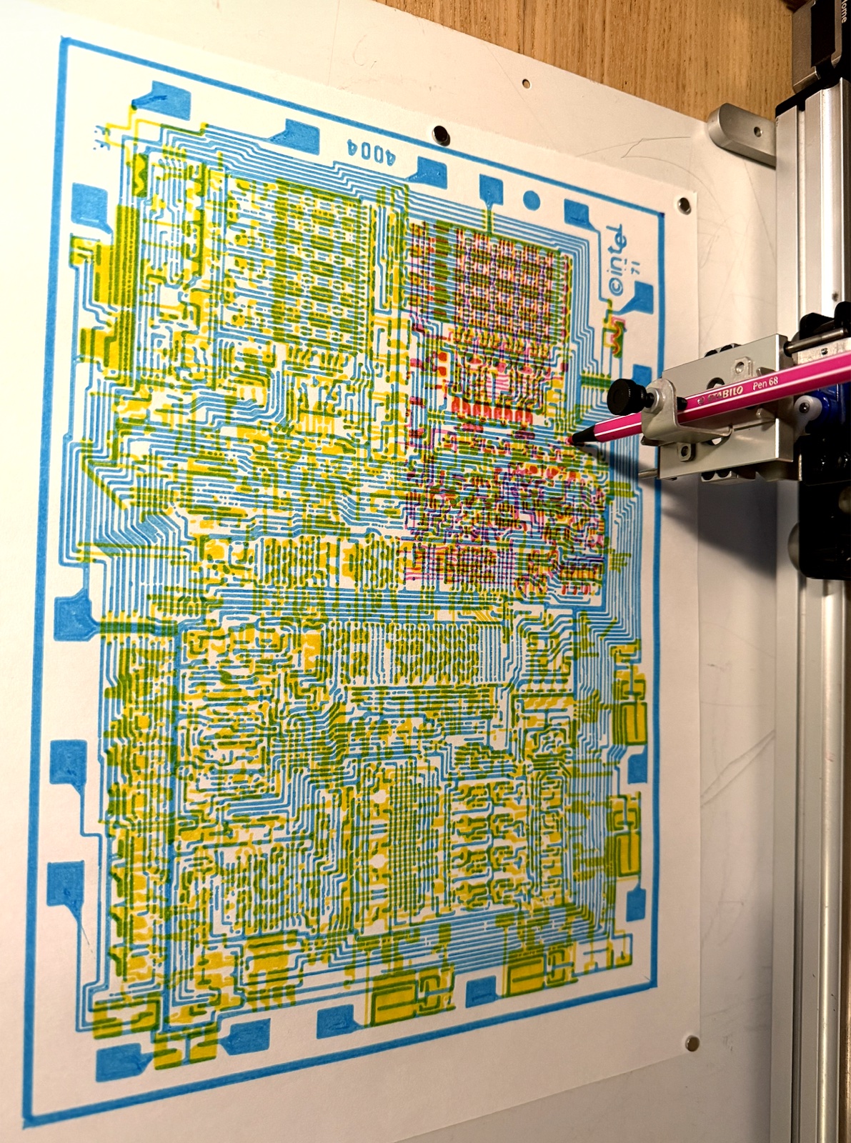
Minotaur is a tool I built from scratch for my pen plotting practice.

I have been plotting on the Axidraw A3 for about 5 years, now, and i love the hardware but was really frustrated at their Inkscape driver. (Inkscape)[https://inkscape.org/] is great, and I usually love FOSS like GIMP. However, for the plots i was trying to do, Inkscape gets slow with tond of nodes, and the actual plotting gui just freezes the app while it’s plotting, and doesn’t provide any feedback. I wanted:

Pause / resume
No GUI freezing
Change speed, accel, pen up/pen down in realtime
see realtime progress
millions of nodes with no lag
faster path optimisation

Other stuff inkscape doesn’t do, that would be cool:

first-class image handling
basic image processing and cleanup
faster image to vector tracing, more options

I don’t need full inkscape featureset either, and I know I can definitely render millions of nodes at 60fps. Especially if I don’t need to manually edit each one. I started with a web interface using Web Serial API but eventually ran into a performance wall when using javascript, and didn’t feel like doing some complicated rust/c++ -> webassembly thing. So i decided to go full C++ / OpenGL / imGui.

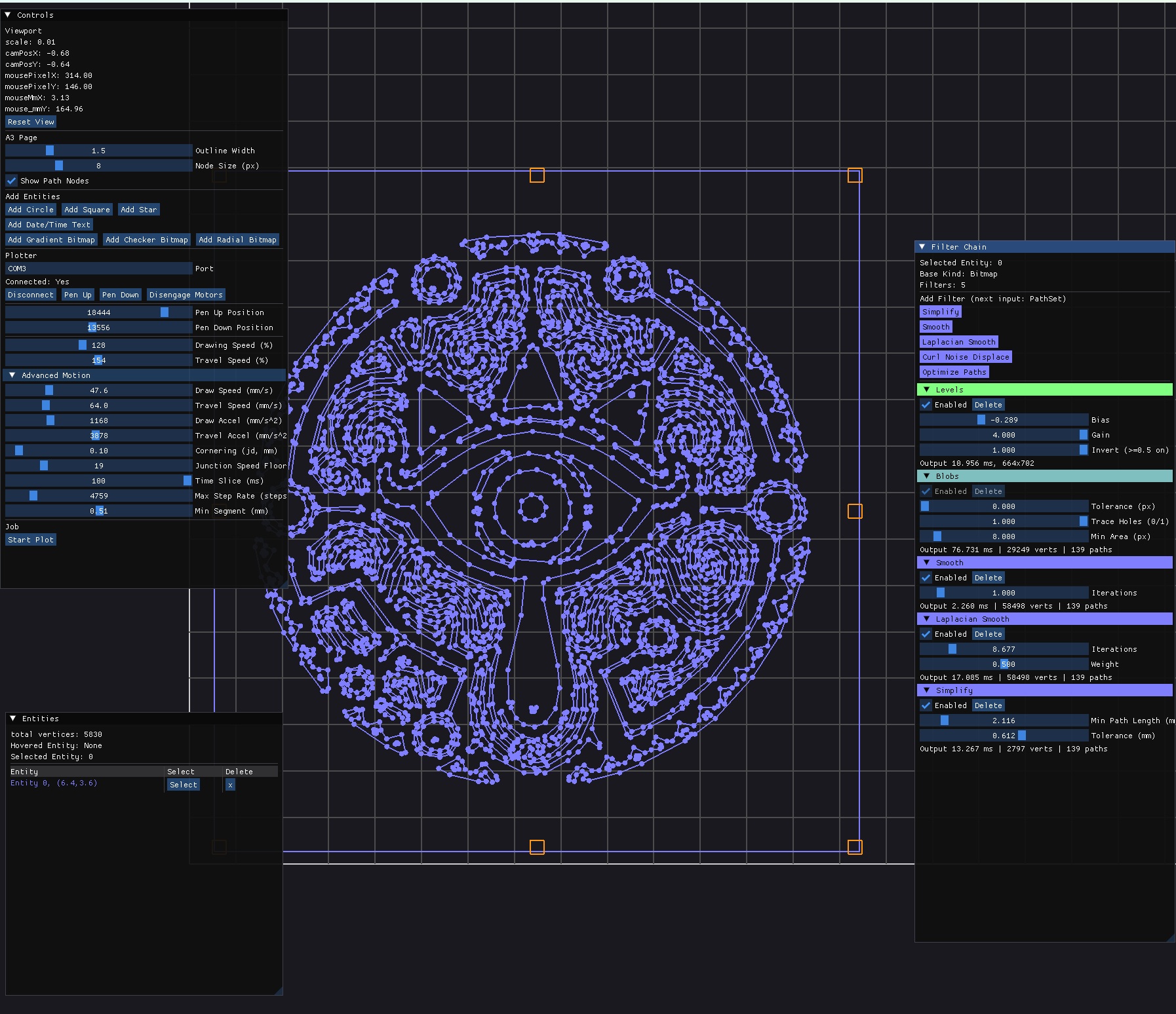
So i designed this around a “filter chain” - where the plot itself starts out as an image, and has these modular building lbocks that can take different types of data and transform/filter it into something that’s plottable.

The core idea is a nondestructive, node-style processing pipeline, i had a bunch of python scripts to modify paths and generate jsons at one point, but it’s much easier to work on it all live! I love realtime!

Architecture

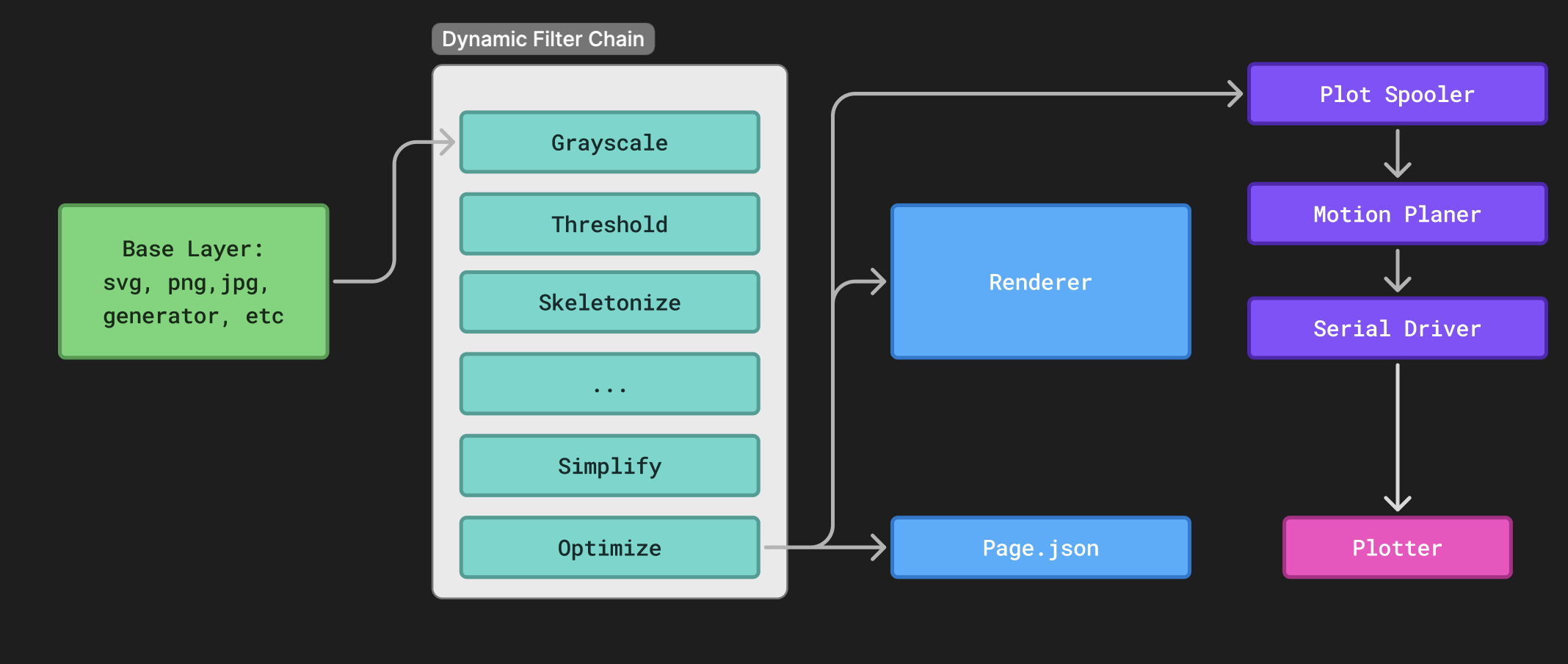
Generator -> Configurable Filter Chain -> Plot Spooling -> Serial connection

Example data flow:

The PageModel has “entities” with a transform and a pathset, or image. The Filter chain is a list of Filters, which output one of these types, and dynamic parameters which can control how it filters the data.

Data Types

Bitmap — 8-bit grayscale row-major. General image format.
FloatImage — 32-bit float, rendered with a colormap. I currently just use this for distance field experiments.
ColorImage — RGB 8-bit interleaved, used for color picking, general “input” format
PathSet — Vector polylines in mm coordinates. A list of list of Vec2.

Filters are type-checked at chain construction time. A filter that takes a Bitmap and outputs a PathSet can’t be placed after a filter that outputs a FloatImage. The system validates this when you add or reorder filters in the UI.

Generators

Instead of importing an image, you can generate content procedurally. I will definitely add more, eventually maybe even a javascript interpreter or sometihng to do some fully generative plots. But right now this is mainly a plotter program, not really where you’re going to do a ton of “generative” type stuff.

SVG Import — Parses SVG files via nanosvg, flattening cubic Béziers with adaptive chord-error tolerance.
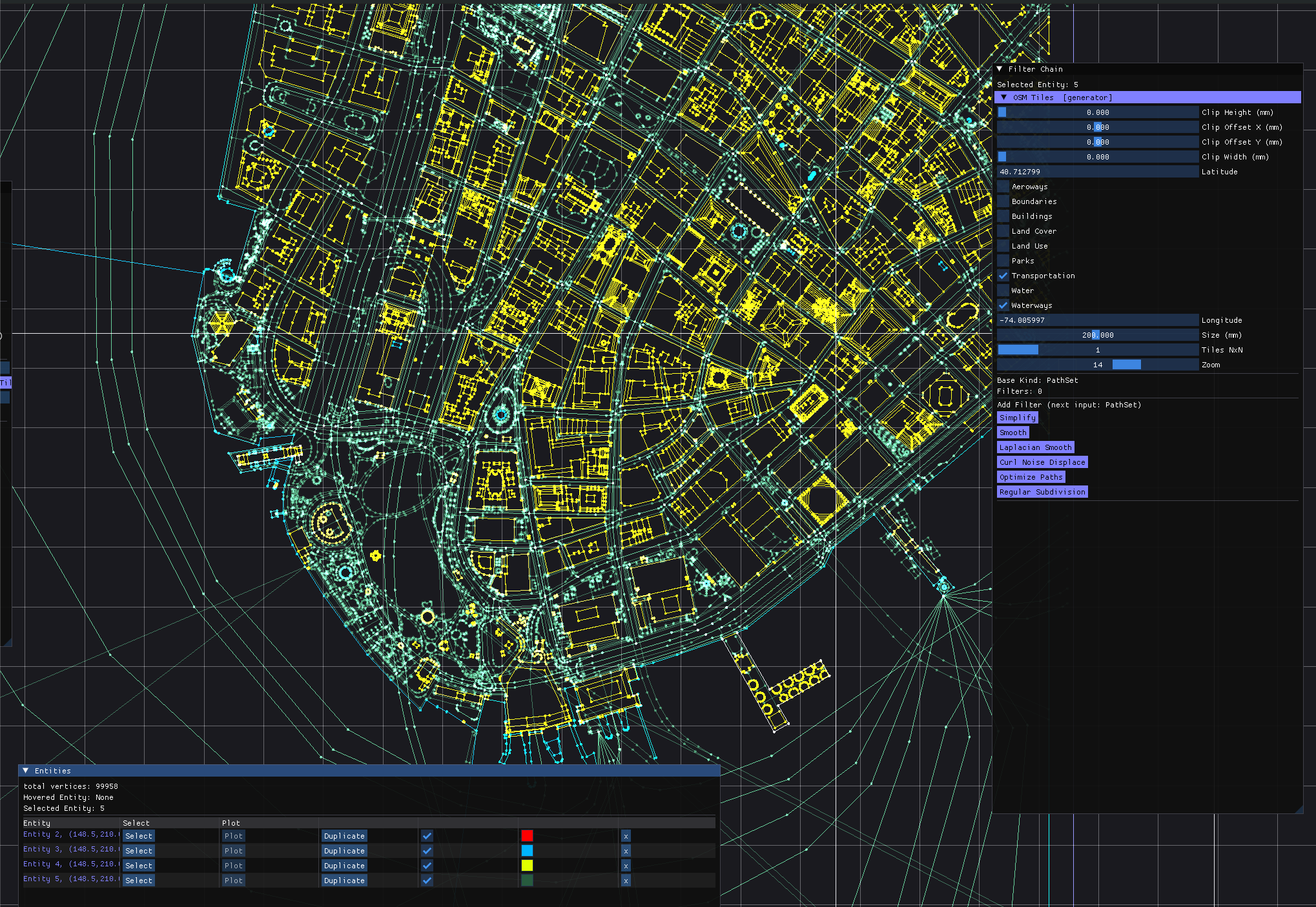
OpenStreetMap — Fetches Mapbox Vector Tiles for any lat/lon region, decodes the the protobuf format, does Mercator projection math, and produces plottable PathSets of streets, buildings, water, parks, and boundaries. The ui is a little clunky but it gets the job done.
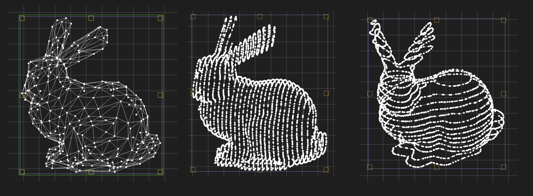
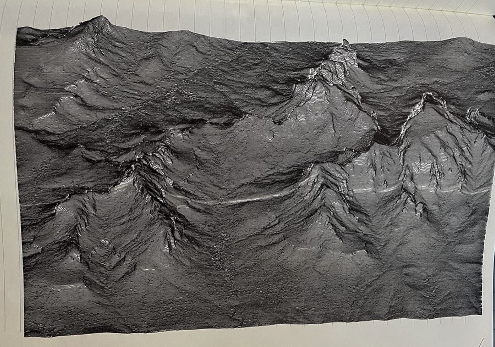
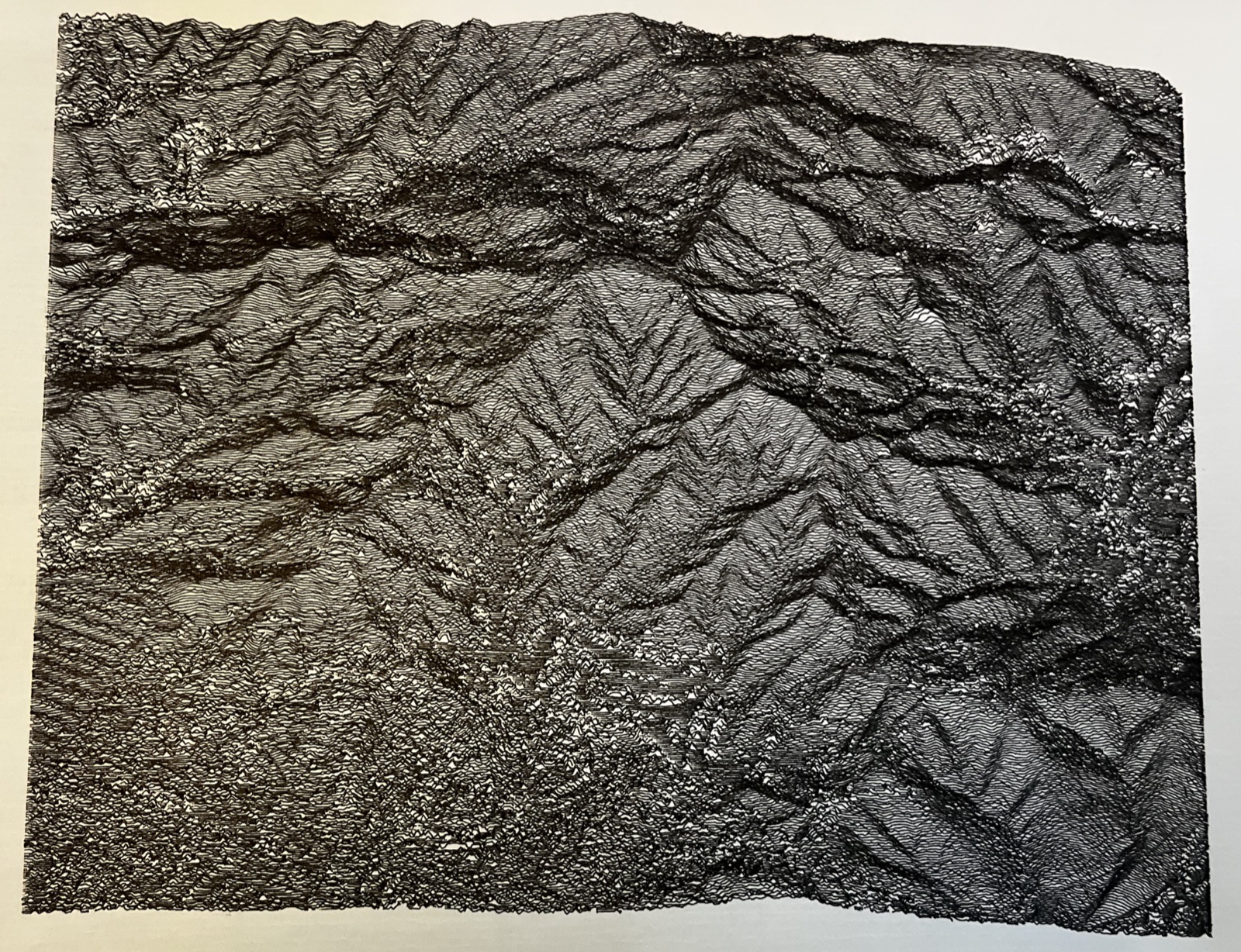
3D Mesh Projection — Loads OBJ files and projects them to 2D with hidden-line removal. The hidden-line algorithm uses scanline rasterization with a depth buffer (GPU-accelerated via OpenGL). It also supports isoline slicing along any axis for a contour-map effect.
Text — basic hershey vector font
Primitives — Circles, stars, grids for testing and geometric compositions.
Image - Can’t be plotted, you need to convert to a PathSet

Detailed topo maps made from the 3D model -> isoline workflow

Bitmap -> Bitmap Filters

Sometimes you might need to clean up the bitmap before you run a trace.

Color Picker - convert RGB to binary grayscale, by threshold to a specific color. useful when you have different pen passes for different areas. Grayscale just turns RGB->gray.
Threshold, Levels, CLAHE (adaptive histogram equalization), Blur, Rotate. These have some fancy SIMD vector instructions when appropriate.
Edge Detection — Canny with configurable thresholds and Gaussian prefiltering.
Erode, Dilate, and Skeletonize. The skeletonizer extracts the medial axis of black regions down to single-pixel-wide skeletons, which produce clean single-stroke paths. I totally just stole the algorithm from scikit-image https://scikit-image.org/docs/0.25.x/auto_examples/edges/plot_skeleton.html

Bitmap -> PathSet Filters

This is where the interesting stuff happens. Theres a lot of different ways to try to get an image to a path, and none of them are good in general, depends on the content.

Binary operators

These run on a black/white binary image. If the input is grayscale, it will just do a threshold.

Blobs - this is a simple BFS flood-fill. I spent some time optimizing this, but it’s still kind fo slow for large images. Just draws an outline for connected components, with optinal hole-filling.
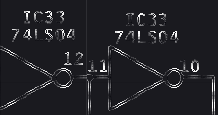
Trace this is just a greedy black-pixel-connector. It works well if you have run a skeletonize filter before, or have very thin lines in your image.
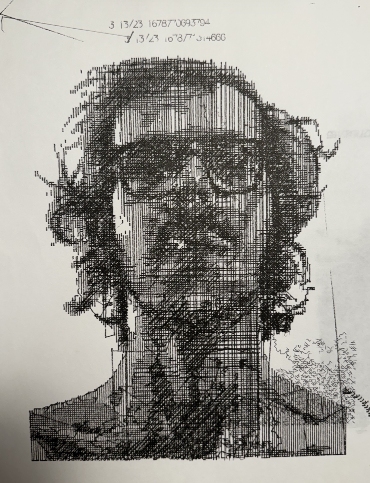
Line Hatch: just Parallel hatching at configurable angles. Simple but effective for shading. I also like to layer multiple plots with varying thresholds to get a full “crosshatching” effect.
Flow Field Hatch: Hatching that follows the image gradient direction (computed via Sobel filters or distance field tangents). Lines curve to follow the contours of the image rather than running in straight parallels. This doesn’t totally work right, still in development.
Concentric Outlines: Generates contours at fixed intervals. This uses the distance field technique, but also is kind of in development. I wanted some more coherent “trace” type paths, but for fatter line images (multiple pixels wide).

Grayscale operators

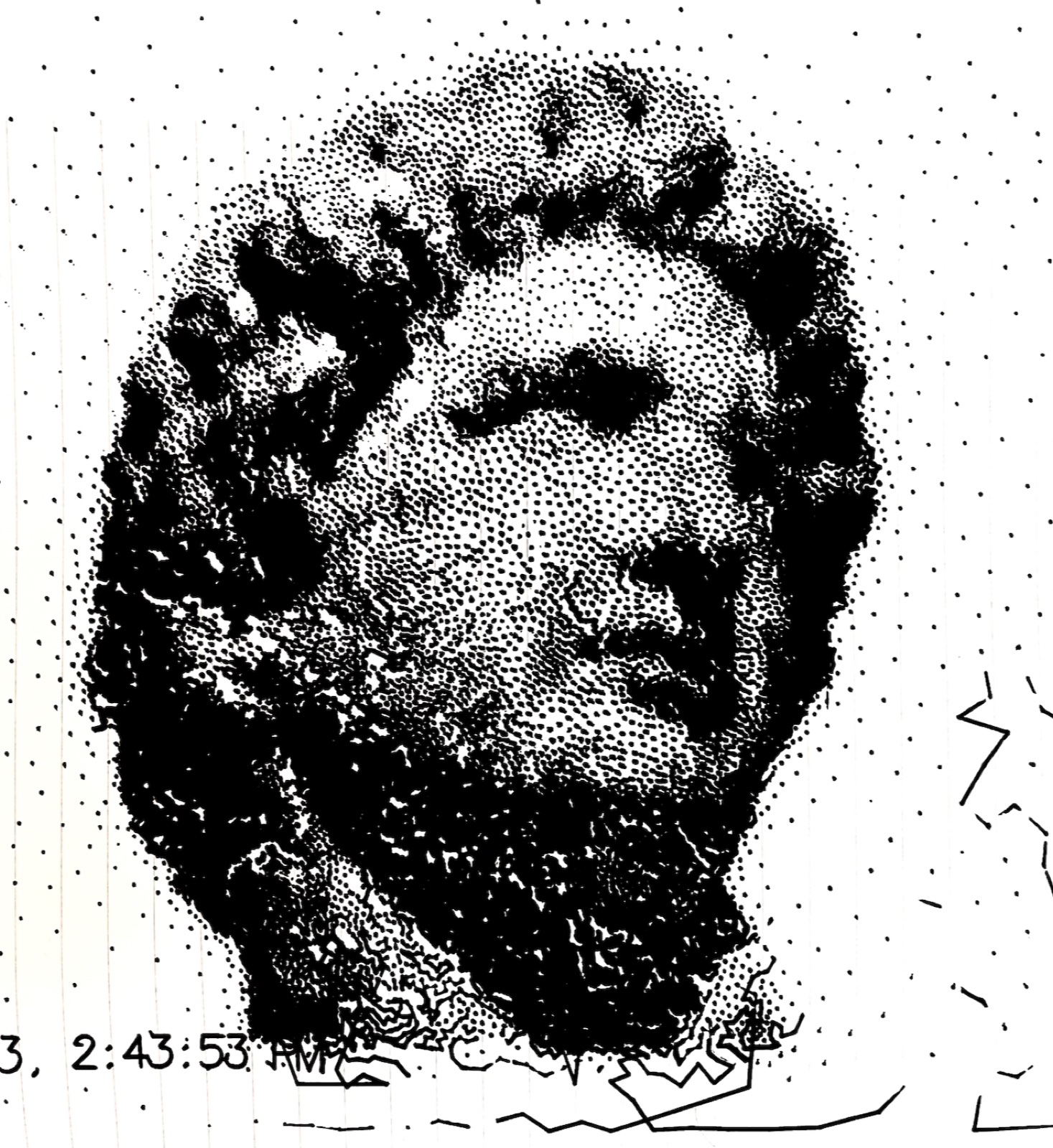
Voronoi Stippling: Lloyd relaxation on 100k+ seed points to produce density-weighted dot distributions. This gives a hand-stippled look where darker regions have tighter dot clusters.
Flow Snake: This is kind of like the physarum algorithm. There is an “agent” which crawls around on the page and “eats” the ink, which increases the value of the pixel and surrouding area using a gaussian. Then, it moves to the darkest area in the range of its sensors (angle and distance is configurable), and repeats. Still haven’t dialed this one in but i have made some cool proof of conecpts.

PathSet -> PathSet Filters

Once you have vector paths, these filters clean them up for plotting. Maybe one day this will be automatic, but it’s nice to be able to tune all the knobs to get it to have the amount of detail / smoothness you want.

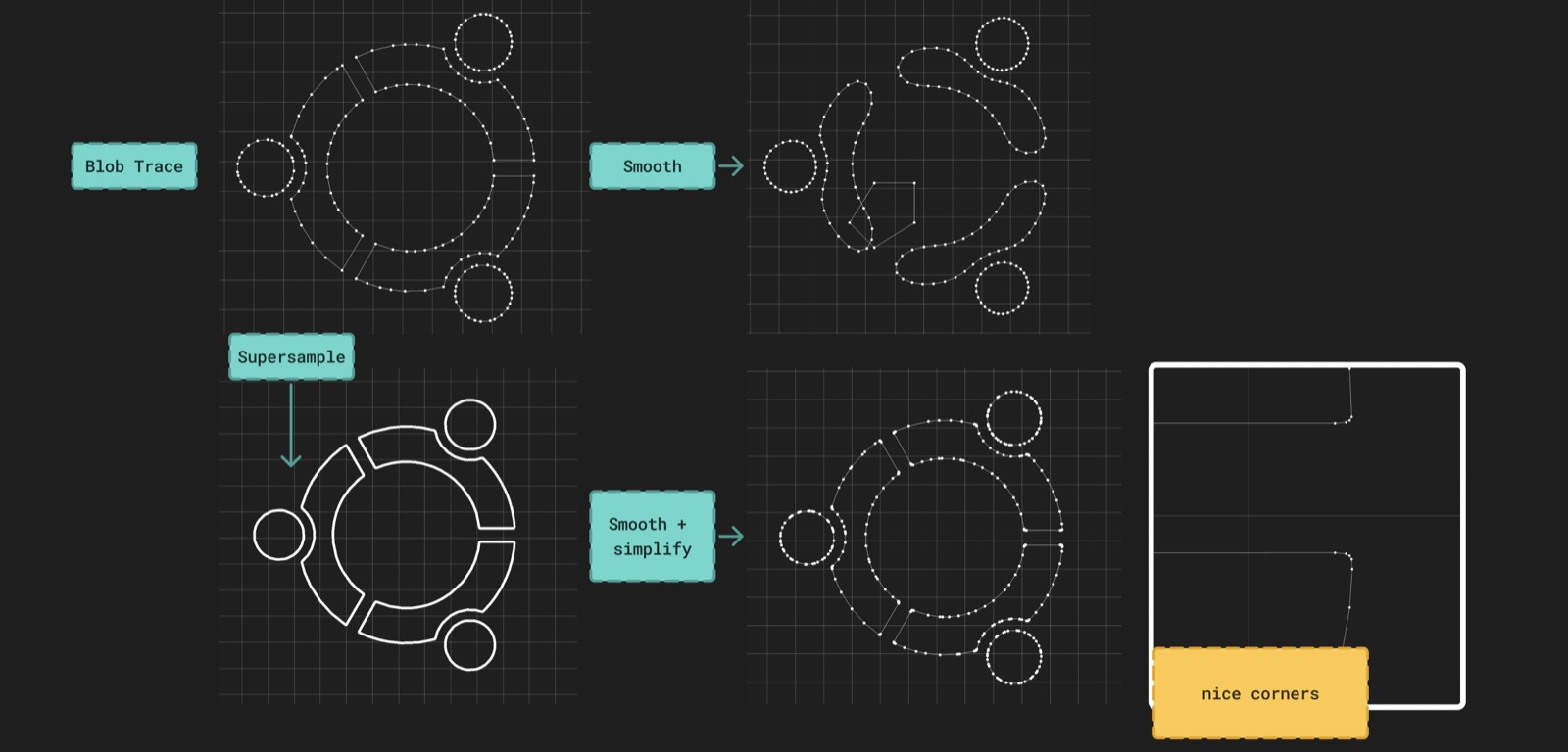
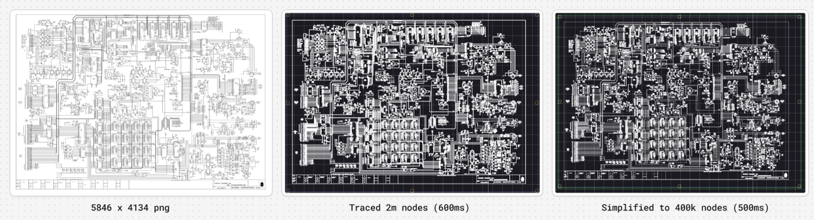
Simplify — Ramer-Douglas-Peucker polyline simplification with minimum segment length culling.
Laplacian Smooth - moves vertex to a weighted average of neighbors. There’s controls for Iterations and amount.
Subdivide — Ensures a maximum distance between consecutive points. This is good to run before a laplacian smoothing so it doesn’t move the
Smooth — Chaikin subdivision makes a ton more points, so i don’t really use it much.

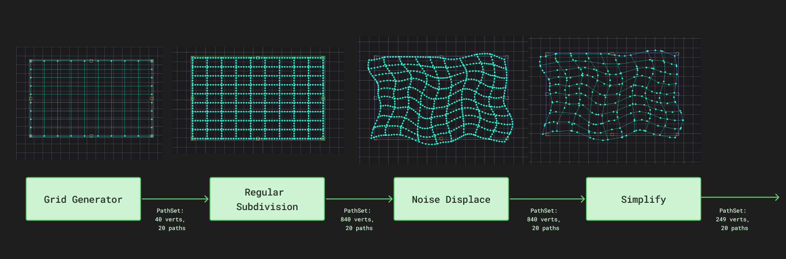
Curl Noise — Perlin noise displacement with octave-based control. Adds organic wobble to paths. I thought this would be more useful than it was, but can make things look a little more natural. I thought eventually this could be more a a “generative” flow where you can make all kinds of cool plots with different filters on generators, but haven’t fully implemented any of those floes yet.

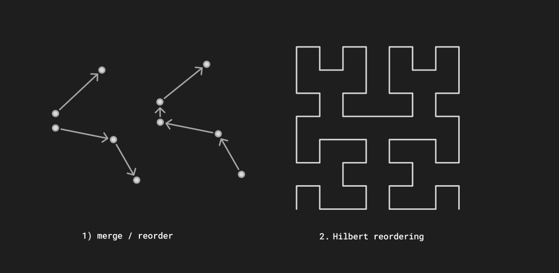
Optimize — Path reordering and merging to minimize total pen-up travel distance. This is kind of traveling salesman problem, but i just use a KDTree and do the greedy solution. An unoptimized plot can easilt have more pen-up traveling than pen down plotting time!

Nearest-neighbor greedy search (fast, good enough, use kD tree)
Hilbert curve ordering which maps 2D path positions to a 1D space-filling curve index. This makes it easier to see the plot progress. I ensure that each cell of a hilbert curve is finished before we start plotting things in aother cell.

Performance

I have tried to pay close attention to making the whole thing efficient and performant from the beginning so we can easily handle millions of nodes and 4k images.

Filter Chain Caching

Each filter’s output is cached with a generation counter. When you change a parameter, only that filter and everything downstream gets recomputed. The evaluation runs on a background thread so the UI stays responsive even during expensive operations like Voronoi stippling or mesh projection. The output accessor is non-blocking during editing and blocking when you actually spool a plot.

Motion Planning

This was the most surprising thing I encountered, i was getting really shit plots with my first custom serial driver. Gowing slow was ok, but I realized the motor can’t instantly accelerate and if you tell it to move to a coordinate and then stop at high velocity, it’s going to have some kickback or wiggle and your plot’s going to look bad.

The solution is a forward-backward velocity pass. This was based on the Sunny Jeon’s cornering algorithm (2011) and the motion planner from the Windell Oskay’s axidraw plugin

Basically, you want to slow down on corners, and saccelerate smoothly when starting and stopping! Simple enough, but makes a huge difference in plot quality.

Serial Streaming

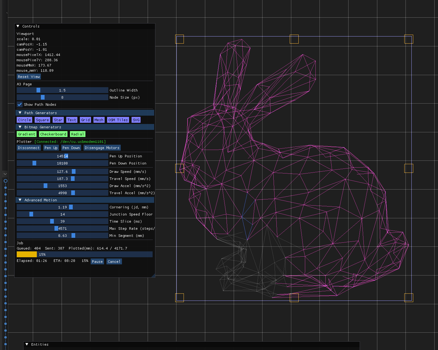
The AxiDraw’s EBB controller has a small command buffer, so the host has to stream commands in real time without gaps (which cause visible pen hesitation) or overflow (which drops commands). The PlotSpooler runs a background thread that has 1s of commands queued up. That way, the frontend can still be responsive, you can see the live plot progress overlaid on the plot.

sheltron